Analyzing liquor sales in Iowa
Iowa State has created a data set for sales of all stores in any brand of liquor. The data set is reachable from here. The data set holds quite detailed information about each sale done in Iowa since January 1, 2012. We can use the set to examine Iowa’s drinking pattern in terms of popular liquors, popular stores and etc. In this post, I will show my work on the dataset, but the special part of this article is what I use to get and visualize the information more than what I do. So, let’s start over like I do when I deal with the Liquor dataset. This is the first time for me to use Rakam so I’m just getting familiar with the concept of Rakam.
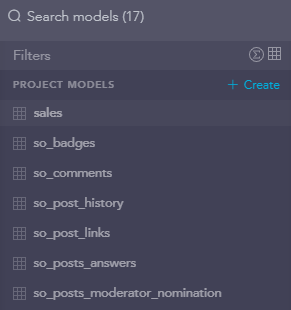
First, you need a project in your rakam account. In the project, you have a model or models. The models represent tables of your database. So creating a model is connecting a database table to rakam.

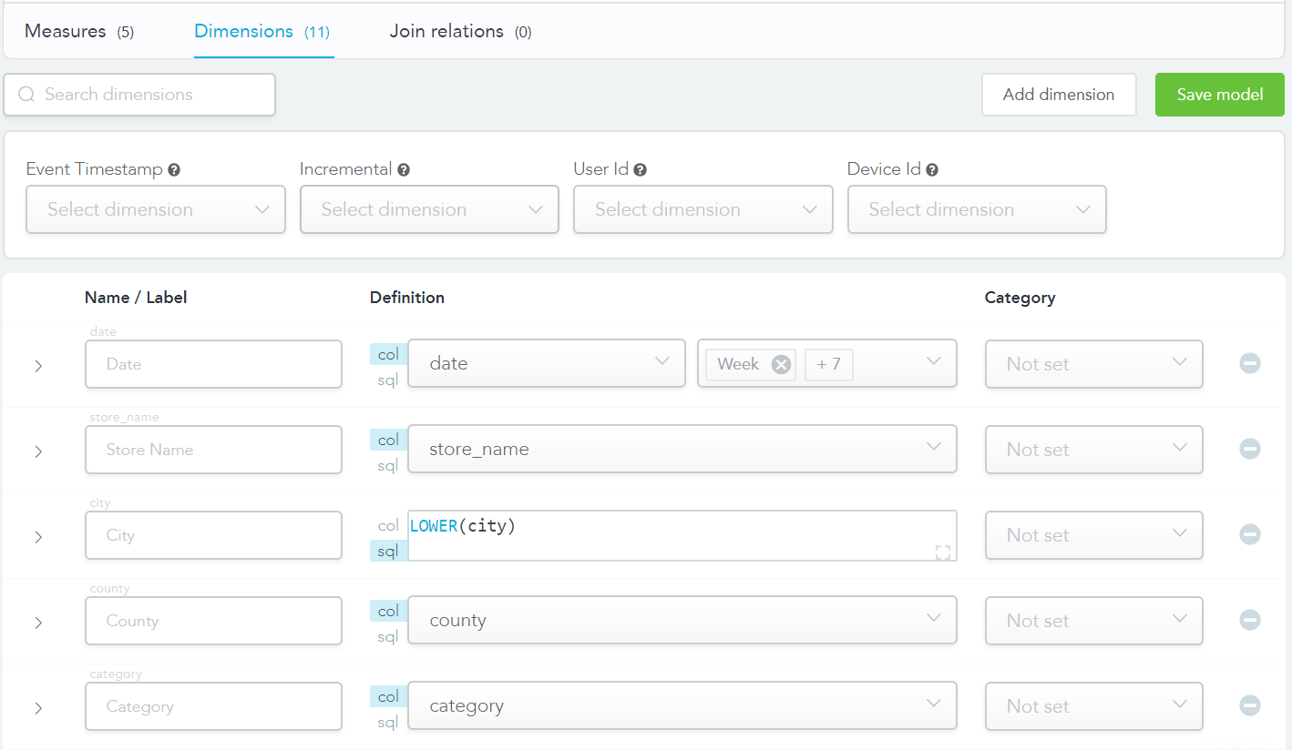
Every model can be named independently from it’s original table name. Also, writing descriptions and categorizing are possible for models. For each model you need to manage measures, dimensions and join relations. Mostly, these three concepts determine what you can do in rakam with your dataset. The most core one is the dimensions. Dimensions directly correspond to columns of the table.

Columns of the table are listed there and remove or add columns for the model. For example, in the original table of the Liquor dataset, there is a column named ‘Store_number’, but you can’t find it among model dimensions because I thought it is not necessary for my work so I removed it. This removing operation does not affect the original table. If necessary, you can do some pre-processing on the value of the dimension’s column on the SQL basis. If you see the dimension named ‘City’ unlike the others it has some SQL code in it’s definition part. City names were not recorded uniformly in the table. For example, there are two different rows that have the city value of ‘Waterloo’ while one of them is ‘Waterloo’ and the other one is ‘WATERLOO’. In SQL, these two values will be considered as two different values although they are not. A SQL method ‘LOWER()’ can solve this problem and in rakam we can use this method in our model for the corresponding dimension. Other than these, you can categorize the dimensions.
The second part of the model is measured. In measures, you define measures based on dimensions of the model. These measures can be count, unique count, sum, minimum, maximum, average and approximately unique of the selected dimension.
In also here, you can pre-process values. As you can see the ‘Max Sales In Bottle’ measure in the image, works on sum of ‘bottle_sold’ column values of the model. Lastly, you can create a join relation for your model. This is directly the same as the SQL’s join relation. Since liquor database has only one table, I didn’t use this part to create any join but to give an explanation, you need to select the target of the join, type of the relation, type of the join and specify the corresponding dimensions as the ‘ON’ part in the SQL code. That’s all for a model representation of tables in rakam. In broad speaking, you define what you need or what you will use in the journey of discovering your dataset.
Now it is time to do some exploration. Also, you can still go back to the model screen and edit your models. In exploration, you have 4 different options as Segmentation, Funnel, Retention, and SQL. Segmentation is the most basic one. In segmentation, you can build queries. First, you need to select a model that you want to build a query on. Secondly, you need to select a measure of that model. The measure corresponds to the value that you want to select in the query. If you want, you can group the by one or more dimensions. Also, you can divide the result into segments by selecting dimensions as pivots. And lastly, you can add filters to your query which directly corresponds to `WHERE` part of queries. Here is an example of segmentation.
I built a segmentation analysis for annual total bottle sales of each store. I measured ‘Total Sales in Bottle’, grouped by ‘Year of Date’, pivoted by ‘Store Name’. To run this query simply click the blue ‘Query’ button on the upper right side of the screen and your query is run. So far, we have a query that is running and we didn’t write any SQL yet we built the query. This means you don’t have to really know SQL anymore.
The results of the query can be seen in the previous figure. Below, result table of the query is shown. Above it, there is a chart that represents the same values in the result table. Results show that from 2012 to 2018, the store named ‘Hy-Vee #3 / Bdi / Des Moines’ sold the most bottles. But so far in 2019, ‘Central City 2’ beats it with almost 20.000 bottle difference. So we can assume that ‘Hy-Vee #3 / Bdi / Des Moines’ is the most popular liquor store of Iowa.
The dashboard is the area that you can store and exhibit any kind of analysis you have done in rakam. You can put your results there either as a chart or table. It is possible to customize the dashboards by resizing and relocating elements in it. Here is a part of my dashboard that I did for the Liquor dataset.
When I see this dataset, I wondered which store sold which brand of liquor the most. For this particular one, I choosed writing a SQL query. This is also possible in rakam. In the explore part there is an option to do your analysis by pure SQL. Here is my query that I wrote on rakam and a small piece of the result.
SELECT DATE_TRUNC(t1.date,MONTH) AS date, t1.store_name, t1.item_description
FROM(
SELECT DATE_TRUNC(date, MONTH) AS date, store_name, item_description, SUM(bottles_sold) AS totalSold
FROM sales
GROUP BY date, item_description, store_name
) AS t1
JOIN(
SELECT DATE_TRUNC(date, MONTH) AS date, store_name, MAX(totalSold) AS maxSold
FROM(
SELECT DATE_TRUNC(date, MONTH) AS date, store_name, item_description, SUM(bottles_sold) AS totalSold
FROM sales
GROUP BY date, item_description, store_name
)
GROUP BY date, store_name
)AS t2
ON t1.date = t2.date AND
t1.totalSold = t2.maxSold AND
t1.store_name = t2.store_name
GROUP BY t1.date, t1.store_name, t1.item_description
| Date | Store_name | Brand |
|---|---|---|
| 2015-12-01 | New Star Liquor / Lafayet / Waterloo | E & J Vs Brandy |
| 2016-01-01 | Casey’s General Store #1125 / Humest | Jim Beam |
| 2018-05-01 | Brewski’s Beverage | Fireball Cinnamon |
| 2018-07-01 | Todd’s | Fireball Cinnamon |
Here is rest of analyses that I do on the dataset through rakam.
In the above image, you can see the annual sales of stores in the dollar. It is clearly seen that sales increased every year. After the year 2017, the store marked with the orange, Costco Wholesale, may be closed because sales dropped down to zero. Also, charts show that the top seller until 2019 is Hy-Vee #3 which can be also considered as the most popular store.
In the below figures, you can find sales values in the bottle for annual and monthly basis with different chart representation.
Although these tables are based on store sales, we can have an idea about alcohol consumption in Iowa. Also, we can find the favorite brand among citizens of Iowa. Here is the chart that shows the total sales of brands in years.
The result shows that, until ‘Black Velvet’ is the most popular one but in recent years, it shared the first place with ‘Fireball Cinnamon’.
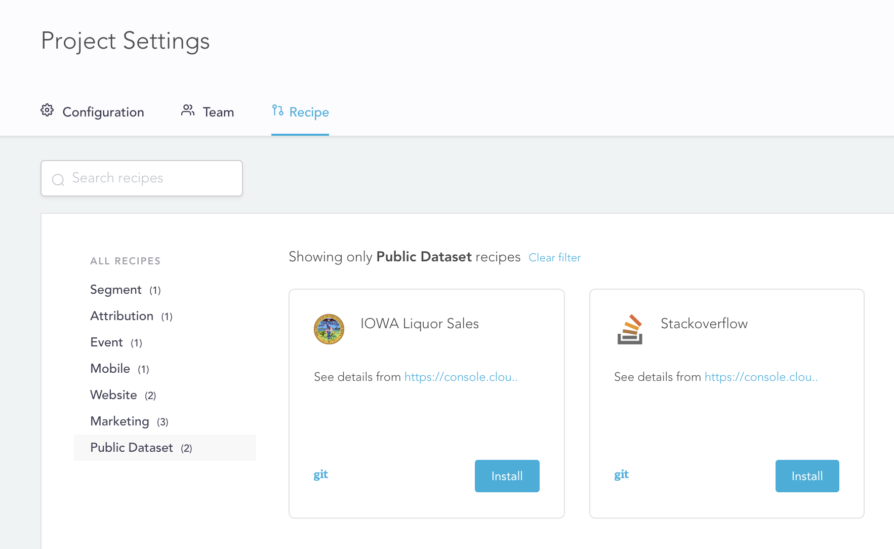
For these analyses, I also used Segmentation and SQL features of rakam. I created a recipe from my work and dashboard on rakam. You can get the recipe from github by the following link https://github.com/rakam-io/recipes/tree/master/gcloud-public-dataset. Also, you can get it on rakam’s recipe page by searching name of the dataset. Here is what you should look for.

It seems there is a lot more that rakam can provide but because of the dataset’s simplicity, I was not able to try and test them. But I want to use rakam more in my future analyses.
