Building Funnel Analysis in SQL vs. Match Recognize

Fundamentally, aggregating event data to the user level enables us to look at how users progress through a particular website experience. As an example, we’ll demonstrate a typical e-commerce flow and what kind of insights we can gain.

Photo by Kelly Sikkema on Unsplash

The application funnel: a walk-through

Consider the user experience at an online storefront like Amazon, Etsy, Target, etc. As a consumer, I would sign up, browse products, and proceed through to checkout. During checkout, I am asked to enter specific details to allow me to complete the order such as my address and subsequently payment information.

When integrating a tool like Snowplow or Segment into an application (like a storefront), the output data is an event stream of user behavior at different points in time. There will be button clicks and page views which, with the right context, can be put into an order to create the “funnel”.

Consider a table event_data, with one row being one event in time: a typical time series.

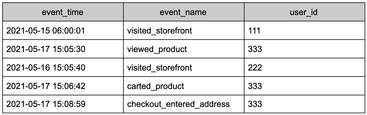
Without further aggregation, this table is very hard to digest. You can imagine the size of this type of table is for a popular site like Etsy or Target, considering the number of users that click on the site every hour; importing that large of a table directly into a BI tool has serious performance implications.

So, we aggregate!

From a time-series event data table, the following query shows which users performed particular actions of interest.

create table funnel_analysis as
select
    a.user_id,
    b.signup_time,
    b.platform_source,
    max(case when a.event_name = ‘visited_storefront’ then 1 else 0 end)
        as visited_storefront,
    max(case when a.event_name = ‘viewed_product’ then 1 else 0 end)
        as viewed_product,
    max(case when a.event_name = ‘carted_product’ then 1 else 0 end)
        as carted_product,
    max(case when a.event_name = ‘checkout_entered_address’ then 1 else 0 end)
        as checkout_entered_address,
    max(case when a.event_name = ‘checkout_saw_payment_options’ then 1 else 0 end)
        as checkout_saw_payment_options,
    max(case when a.event_name = ‘checkout_completed’ then 1 else 0 end)
        as checkout_completed
from event_data_table as a
left join user_model as b on a.user_id = b.id
where cast(a.event_time as date) <= date_add(day, 30, cast(b.signup_time as date))
group by a.user_id, b.signup_time, b.platform_source;

Let’s dissect this a bit.

Expanding on the technical details

First, the code queries the event table and joins user properties so we can analyze potential differences between user segments. For instance, the marketing team might want to know if users coming from the Facebook Ads platform behave differently in the storefront than users coming from the Google Ads platform.

To aggregate to the user level, we assign a binary 0/1 value to columns with particular events. With this structure, to evaluate how many users have performed a particular action we can just sum over that column: the result from running sum(checkout_entered_address) will be the total number of users that entered their address at checkout.

Lastly, the event times are capped to within 30 days of signup. The longer the user is on the platform, the more likely they are to have performed a particular action. Without this filter, recent signups will have inherently worse metrics. Now, if looking at users who signed up more than 30 days ago, they have an equal opportunity (read: 30 days) to perform the actions of interest.

What does formatting the data this way give us?

Photo by Suzanne D. Williams on Unsplash

Querying the summary numbers will indicate if there is an obvious drop-off in the flow. For instance, if total_users is substantially higher than visited_storefront, many users are simply signing up but not engaging with the shopping site. This would indicate an opportunity to re-engage users by emailing them for instance.

Alternatively, if checkout_saw_payment_options is much higher than checkout_complete, the provided payment options might not be versatile enough for users to be able to pay successfully. Investigating different payment integrations (like Stripe, Google/Apple Pay, etc) may increase the number of users that actually complete a purchase.

When companies look at “conversion rates”, these are the types of questions they are trying to answer.

Let’s see how querying the funnel_analysis table created above can answer some of these questions.

To start, here’s the highest level aggregation, only giving summary numbers.

select
    count(*) as total_users,
    sum(visited_storefront) as visited_storefront,
    sum(viewed_product) as  viewed_product,
    sum(carted_product) as carted_product,
    sum(checkout_entered_address) as checkout_entered_address,
    sum(checkout_saw_payment_options) as checkout_saw_payment_options,
    sum(checkout_completed) as checkout_complete
from funnel_analysis;

The summary is informative but isn’t indicative of any changing trends. By adding the signup_time or platform_source, we can see if there are other contributing factors to conversions.

select
    cast(signup_time as date) as signup_date, -- or: platform_source
    count(*) as total_users,
    sum(visited_storefront) / count(*) as visited_storefront_percent,
    sum(viewed_product) / count(*) as  viewed_product_percent,
    sum(carted_product) / count(*) as carted_product_percent,
    sum(checkout_entered_address) / count(*) as checkout_entered_address_percent,
    sum(checkout_saw_payment_options) / count(*) as checkout_saw_payment_options_percent,
    sum(checkout_completed) / count(*) as checkout_complete_percent
from funnel_analysis
group by cast(signup_time as date)
order by cast(signup_time as date);

The goal isn’t to look at overall volumes over time of signup, rather the rate at which users complete the user flow. More specifically, taking sum(visited_storefront) / count(*) gives the ratio of the total signed-up users that actually go on to use the storefront. In general, dividing one metric by the metric logically after it in the flow gives conversion ratios. (Technical aside: in many SQL environments you’ll have to cast these as floats explicitly so the division results in a decimal, not a 0 / 1 integer).

In the daily view, performing the division grouping by the day shows how conversion performs over time. If there’s a large product launch on a particular date (such as an introduction of new items in the storefront or new payment options), any changes to the above metrics would be an indicator of the performance of the product.

Similarly, grouping by platform_source would show differences in behavior between how users were sourced and attributed.

Other approaches

There are many ways to look at conversions, and many ways to actually calculate them. Several SQL flavors support the function match_recognize, most notably Snowflake. The function accepts a set of rows as input (the time-series) and detects particular patterns (or events) in the data.

The above analysis can be re-written (while also adding the count metrics) like the below using match_recognize.

select
    a.user_id,
    b.signup_time,
    b.platform_source,
    visited_storefront as visited_storefront_count,
    viewed_product as viewed_product_count,
    carted_product as carted_product_count,
    checkout_entered_address as checkout_entered_address_count,
    checkout_saw_payment_options as checkout_saw_payment_options_count,
    checkout_completed ascheckout_completed_count
from event_data_table as a
left join user_model as b on a.user_id = b.id
where cast(a.event_time as date) <= date_add(day, 30, cast(b.signup_time as date))
match_recognize(
    partition by user_id
    order by event_time
    measures count(*) as actions,
             count(visited_storefront.*) as visited_storefront,
             count(viewed_product.*) as viewed_product,
             count(carted_product.*) as carted_product,
             count(checkout_entered_address.*) as checkout_entered_address,
             count(checkout_saw_payment_options.*) as checkout_saw_payment_options,
             count(checkout_completed.*) as checkout_completed
    one row per match
    pattern(visited_storefront (anything)*)
    define
        visited_storefront as event_name = ‘visited_storefront’,
        viewed_product as event_name = viewed_product,
        carted_product as event_name = carted_product,
        checkout_entered_address as event_name = checkout_entered_address,
        checkout_saw_payment_options as event_name = checkout_saw_payment_options,
        checkout_completed as event_name = checkout_completed
);

Additionally, window functions are extremely helpful in performing aggregations with a filter, resulting in cumulative aggregations. For instance, the simple sum() function used in the examples above can be turned into a window function; running sum(total_users) over (order by signup_time) will result in a cumulative total of users who sign up over time.

Although window functions are a versatile approach, using specific functions within each data warehouse may result in significant efficiency improvements. Snowflake’s match_recognize is designed to optimize for behavioral analysis, like the funnel analysis example in e-commerce.

In the examples, I’ve tried to be warehouse agnostic so they can be generalized. Each warehouse will have its own extra functionality (like match_recognize in Snowflake) which can certainly be leveraged to make time-series easier to work within SQL and significantly more efficient.